Feature Selection for Marketing Mix Modelling using Boruta Algorithm

Any new Marketing Mix Modelling (MMM) project starts with thorough preparation steps: before we even collect and process the input data, we need to decide which data is relevant and could serve as meaningful modelling variables. In the modern world, the problem of data scarcity has been replaced with a new challenge - data abundance. So much data has become available to us that we need help navigating around it and assessing its relevance for specific purposes.

Of course, one possible option is to throw all the variables we have into our MMM model to see which ones get a tangible contribution and then get rid of the factors with zero effect. This might be a valid approach if we have just a few variables available but in real-life situations it is mostly inefficient and could even result in misleading conclusions. So a more robust approach would be to pre-select the factors that are expected to affect our target variable and model only with these features. In machine learning this process is called Feature Selection.

There are several possible methods of doing it. Today we will test an algorithm called Boruta and decide if we can apply it to feature selection for MMM.

What is Boruta?

Boruta is a machine learning algorithm developed by Miron B. Kursa and Witold R. Rudnicki. Based on the Random Forest classification method, it either rejects or confirms the importance of individual features. For each data row, the algorithm creates a shadow feature - a copy of the original feature but with randomly mixed values, so that their distribution remains the same. Then it calculates the importance of the original feature and its shadow with respect to the target variable and compares them to each other. This process is repeated multiple times (by default 100 cycles), each time re-shuffling the values in the shadow feature. At the end, the algorithm compares the importance of the feature to the highest score of its shadows and decides whether the original feature is significant or not. 

As the basis, we used the Sample Media Spends dataset from Kaggle. https://www.kaggle.com/datasets/yugagrawal95/sample-media-spends-data?resource=download

The target KPI in this dataset is “Sales”. The media variables we used are “Google”, “Facebook”, “Affiliate”, as well as “Email” and “Organic”. The breakdown into divisions is not necessary so we dropped the column and grouped the data by week.

Let’s plot the media variables against the target KPI to check for obvious correlations in their development. We need to split Google, Email and Facebook from Organic and Affiliate because of the difference in the impressions scale.

The variables “Google”, “Facebook”, and “Email” seem to correlate pretty well with the Sales. On the other hand, Sales correlation with Organic and Affiliate is not so clear.

Our dataset is still missing context variables. Although some companies might prefer to leave them out in order to maximize the effect of their media, it would be unrealistic to believe that sales are not affected by any external factors or non-media activities so let us add some variables:

• Weather: sunshine hours, wind speed, precipitation and temperature
• COVID statistics: number of cases and deaths
• School holidays: winter, spring, summer, autumn and total, weighted by the population of corresponding regions
• Consumer price index (moving average centered over 5 weeks). 

Moreover, we still need to spice up our dataset - that is, add some events as dummy variables with 1 and 0 values. In our practice, such variables often come into play when the company doesn’t have exact reach or spend data for special events or occasions. We will add three different TV Shows that coincide with slight spikes in Sales.

Boruta Modelling

Let’s proceed with Boruta modelling. We will use RStudio and the dedicated R package for Boruta.

Next we create a dataset based on our input data file.

Unfortunately Boruta doesn’t recognize the time dimension in the data. All the data points are compared within one row of data without any reference to previous or future time points. The columns containing dates are not necessary for modelling, so we will remove them.

It’s important to note that if we want to apply Boruta to our media variables, we need to use adstocked values. Such data is not always available, especially if you are running MMM for the first time ever. Moreover, companies normally prefer to keep all media variables in the modelling, even if there is no obvious correlation to the target variable. Therefore in practice we normally don’t need to include media variables into the feature selection process but we will keep them in our case for testing purposes and assume that our values already include the adstock effect.

Now let’s run Boruta. We will keep the maximum number of runs at the default level of 100 for now and use the value 2 for the argument “doTrace” to keep detailed track of the process. Our Target column is “Sales”.

The algorithm takes just a few moments to run 100 iterations. Let’s check the output.

Here is what we get:

We can also take a look at the statistics:

Our outcome:

Let’s plot the results to have a better overview:

By default Boruta plots the variables on the horizontal axis and the importance values on the vertical axis. The features with confirmed importance are colored green, the ones rejected are red and optionally, there might be a yellow group that’s tentatively confirmed but requires consideration.

Here is our chart:

This chart is more informative and easier to digest than the text outputs we got above. You will see this chart in most resources describing the application of Boruta but in our opinion, it’s a bit hard to read. Moreover, if the variable names are too long, they will get truncated, which might lead to confusion. Let’s change a few things in the code and flip our axes. First we will need some more libraries:

Our code for the chart will look like this:

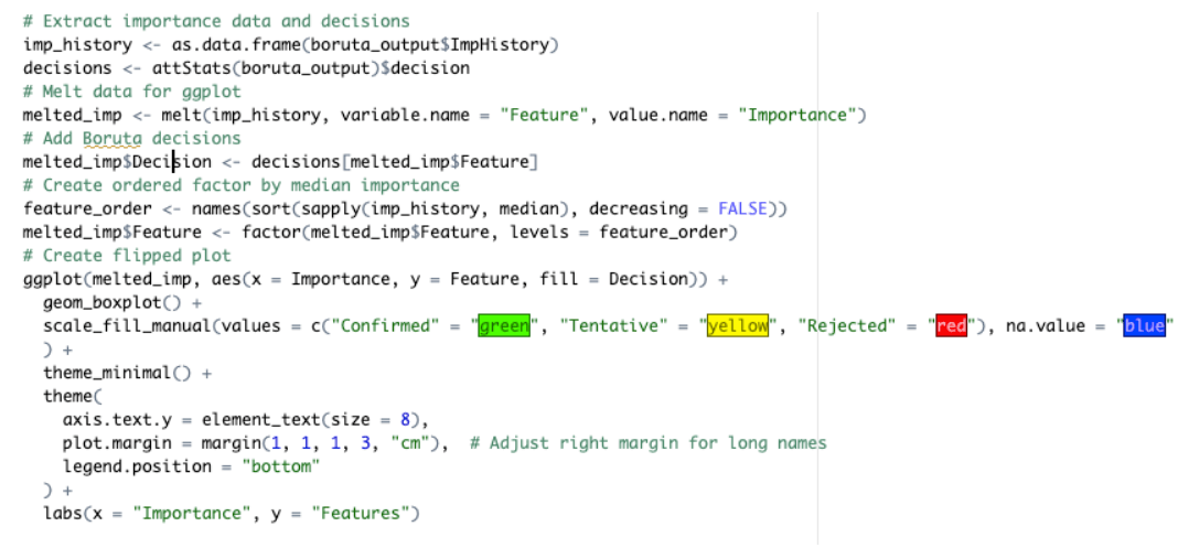
And here is the outcome:

This version of the chart makes it much easier to read and interpret the results.

You can read more about the Boruta R package here: https://cran.r-project.org/web/packages/Boruta/Boruta.pdf

Modelling outcomes

Now let’s look at the chart and draw conclusions about our features:

1. Paid and organic media: All the 5 variables have confirmed their importance, although the Organic one is somewhat behind the rest. Our initial analysis questions the relevance of Organic and Affiliate. In practice, however, companies prefer to include all available media variables into modelling and even a tiny impact is important. So as long as Boruta doesn’t reject the variables, it might make sense to keep them although not all of them produce equal impact.
2. Weather: Sunshine duration and Temperature made it to the final list, whereas Precipitation and Wind Speed seem to be irrelevant.
3. COVID: Both variables, COVID cases and deaths, received very low importance scores and can be discarded.
4. School holidays: Boruta suggests that only autumn holidays have an impact on the Sales, the rest are not important.
5. Consumer Price Index: Although this variable doesn’t get the highest importance score, it’s still in the green group and should be included in the MMM. Even if it doesn’t get a high coefficient, it might help increase the overall accuracy of the model.
6. TV Shows: All the 3 instances received a very low importance score from Boruta, although we saw that each one of them coincided with a small uplift in Sales. Why is that? Our TV Show variables represent a row of data containing one “1” and the rest of the values are “0”. Since the actual variable is compared to shadows where all values except one are zeros but each time sorted in a random order, this comparison is not a valid approach. Even if instead of “1” and “0” we use the actual Reach or Spend figures, but the variable only has one or a couple of non-zero values, Boruta will most likely classify this feature as unimportant.

Based on these results, we can drop irrelevant columns and make our modelling dataset considerably lighter, thus optimizing the MMM process.

Conclusions about applicability for MMM

Although the final outcome of Boruta is quite easy to interpret and operationalize, this method is not a perfect match for Marketing Mix Modelling feature selection. It can be applied with certain limitations and requires expert knowledge. In order to take the delayed effect into account, Paid and Organic Media need to be adjusted with adstock. Moreover, the variables with prevailing zero or missing values, such as dummy variables with one or a few “1” and many “0” values, will most likely get a false negative result from Boruta. In MMM applications, we suggest using Boruta specifically for context variables that have all (or most) non-zero values and span across the entire time range, such as weather data or inflation rate.